Annotation consensus

The pylidc.utils.consensus() utility accepts a list of annotations to produce a single boolean-valued volume of those annotations. It also returns the individual boolean masks for each Annotation, placed in a common frame of reference – i.e., a common bounding box, which is also returned.

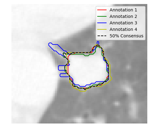
In the following example, we first compute the 50% consensus consolidation of the annotation contours, then we plot them along with the original 4 contours from the 4 different annotations of the nodule:

import numpy as np
import matplotlib.pyplot as plt
import matplotlib.animation as manim
from skimage.measure import find_contours

import pylidc as pl
from pylidc.utils import consensus


# Query for a scan, and convert it to an array volume.
scan = pl.query(pl.Scan).filter(pl.Scan.patient_id == 'LIDC-IDRI-0078').first()
vol = scan.to_volume()

# Cluster the annotations for the scan, and grab one.
nods = scan.cluster_annotations()
anns = nods[0]

# Perform a consensus consolidation and 50% agreement level.
# We pad the slices to add context for viewing.
cmask,cbbox,masks = consensus(anns, clevel=0.5,
                              pad=[(20,20), (20,20), (0,0)])

# Get the central slice of the computed bounding box.
k = int(0.5*(cbbox[2].stop - cbbox[2].start))

# Set up the plot.
fig,ax = plt.subplots(1,1,figsize=(5,5))
ax.imshow(vol[cbbox][:,:,k], cmap=plt.cm.gray, alpha=0.5)

# Plot the annotation contours for the kth slice.
colors = ['r', 'g', 'b', 'y']
for j in range(len(masks)):
    for c in find_contours(masks[j][:,:,k].astype(float), 0.5):
        label = "Annotation %d" % (j+1)
        plt.plot(c[:,1], c[:,0], colors[j], label=label)

# Plot the 50% consensus contour for the kth slice.
for c in find_contours(cmask[:,:,k].astype(float), 0.5):
    plt.plot(c[:,1], c[:,0], '--k', label='50% Consensus')

ax.axis('off')
ax.legend()
plt.tight_layout()
#plt.savefig("../images/consensus.png", bbox_inches="tight")
plt.show()