The Annotation class
A pylidc.Annotation object belongs to a pylidc.Scan object:
import pylidc as pl

ann = pl.query(pl.Annotation).first()
print(ann.scan.patient_id)
# => LIDC-IDRI-0078
Jump to:
Querying annotation feature values
The queryable attributes for Annotation objects are the characteristic values assigned by the particular annotating radiologist:
anns = pl.query(pl.Annotation).filter(pl.Annotation.spiculation == 5,
                                      pl.Annotation.malignancy == 5)
print(anns.count())
# => 91
Note
Not all of the class attributes are queryable! Some attributes are actually computed properties. You can determine this by, for example, examining the object type for the class:
print(type(pl.Annotation.lobulation))
# => <class 'sqlalchemy.orm.attributes.InstrumentedAttribute'>
# => ^^^ queryable because it's an sqlalchemy attribute.

# Whereas ...
print(type(pl.Annotation.Lobulation))
# => <type 'property'>
# ^^^ not queryable because it's a computed property
The lobulation attribute is the numerical value assigned by the annotating radiologist, whereas the Lobulation attribute is a property that encodes the numerical value to the semantic string representation.
Each of the characteristic values are the numerical values assigned by the annotating radiologist. Alongside each of these attributes is a corresponding computed property that gives the semantic interpretation of the numerical value for a given characteristic:
ann = pl.query(pl.Annotation)\
        .filter(pl.Annotation.malignancy == 5).first()

print(ann.malignancy, ann.Malignancy)
# => 5, 'Highly Suspicious'

print(ann.margin, ann.Margin)
# => 2, 'Near Poorly Defined'
The names of these characteristics are found in pl.annotation_feature_names:
('subtlety',
 'internalStructure',
 'calcification',
 'sphericity',
 'margin',
 'lobulation',
 'spiculation',
 'texture',
 'malignancy')
All of these characteristics values and strings can be quickly viewed by:
ann.print_formatted_feature_table()
# => Feature              Meaning                    #
# => -                    -                          -
# => Subtlety           | Obvious                  | 5
# => Internalstructure  | Soft Tissue              | 1
# => Calcification      | Absent                   | 6
# => Sphericity         | Ovoid/Round              | 4
# => Margin             | Near Poorly Defined      | 2
# => Lobulation         | Near Marked Lobulation   | 4
# => Spiculation        | No Spiculation           | 1
# => Texture            | Solid                    | 5
# => Malignancy         | Highly Suspicious        | 5
We can also query directly for the attributes themselves, rather than the entire Annotation object:
svals = pl.query(pl.Annotation.spiculation)\
          .filter(pl.Annotation.spiculation > 3)

print(svals[0])
# => (4,)

print(all([s[0] > 3 for s in svals]))
# => True
Contour-derived data
The pylidc.Contour class is almost never used directly, but only
through the pylidc.Annotation object to which the contours belong.
They can be accessed directly, however, via:
ann = pl.query(pl.Annotation).first()
contours = ann.contours

print(contours[0])
# => Contour(id=21,annotation_id=1)
The diameter, surface_area, and volume attributes are all, for example, computed properties that use the contour data for a particular Annotation:
print("%.2f mm, %.2f mm^2, %.2f mm^3" % (ann.diameter,
                                         ann.surface_area,
                                         ann.volume))
# => 20.84 mm, 1242.74 mm^2, 2439.30 mm^3
A boolean-valued volume can be obtained that is 1 to indicate nodule and 0 to indicate non-nodule:
mask = ann.boolean_mask()
print(mask.shape, mask.dtype)
# => (34, 27, 6), dtype('bool')
Note by the shape of the volume that the boolean-valued mask does not occupy the entire extent of the CT image volume (which is 512 x 512 x num slices). Rather, the boolean mask sits within the computed “bounding box” of the nodule, which is the computed extent of the contour indices of the annotation.
The pylidc.Annotation.bbox() method returns a tuple of slices
corresponding to the nodule bounding box indices. This can be used to
easily index into the NumPy CT image volume:
bbox = ann.bbox()
print(bbox)
# => (slice(151, 185, None), slice(349, 376, None), slice(44, 50, None))

vol = ann.scan.to_volume()
print(vol[bbox].shape)
# => (34, 27, 6)
Note that both the pylidc.Annotation.boolean_mask() and the
pylidc.Annotation.bbox() methods accept a pad argument which
can be used for adding context about the nodule.
We can also get the physical dimensions of the bounding box:
print(ann.bbox_dims())
# => [21.45, 16.90, 15.0]
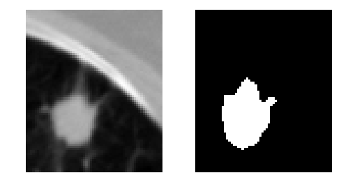
Annotation visualization
The pylidc.Annotation class provides two direct convenience functions
for visualization annotation data which we will show below; however,
let’s first continue the
pylidc.Annotation.boolean_mask() and
pylidc.Annotation.bbox() examples from above to provide a
visualization of the annotated nodule:
import pylidc as pl
import matplotlib.pyplot as plt

ann = pl.query(pl.Annotation).first()
vol = ann.scan.to_volume()

padding = [(30,10), (10,25), (0,0)]

mask = ann.boolean_mask(pad=padding)
bbox = ann.bbox(pad=padding)

fig,ax = plt.subplots(1,2,figsize=(5,3))

ax[0].imshow(vol[bbox][:,:,2], cmap=plt.cm.gray)
ax[0].axis('off')

ax[1].imshow(mask[:,:,2], cmap=plt.cm.gray)
ax[1].axis('off')

plt.tight_layout()
#plt.savefig("../images/mask_bbox.png", bbox_inches="tight")
plt.show()
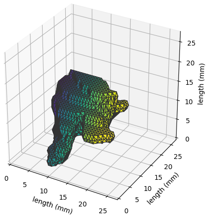
Surface visualization
The nodule surface (as obtained by a single annotator) can be visualized in three dimensions by invoking the following:
ann = pl.query(pl.Annotation)\
        .filter(pl.Annotation.lobulation == 5).first()
ann.visualize_in_3d()
which appears as:
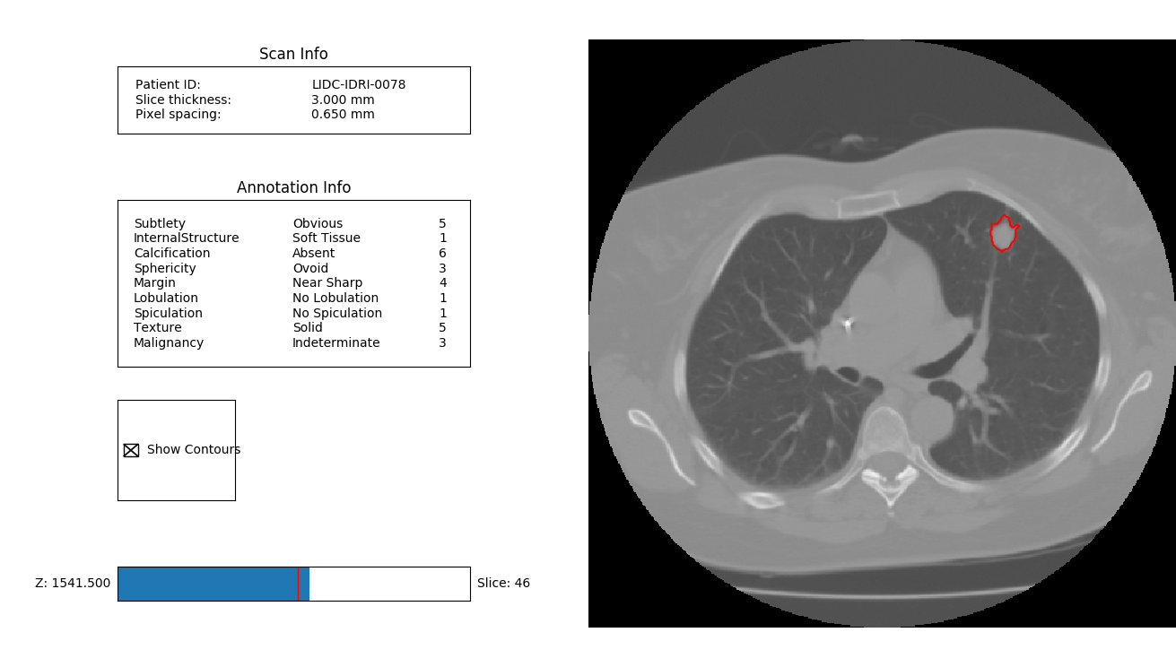
CT visualization
The contours can be visualized interactively on top of the CT image data:
ann = pl.query(pl.Annotation).first()
ann.visualize_in_scan()
which appears as: